Zernike polynomials

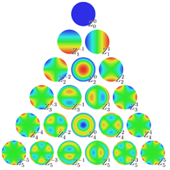
In order to manually introduce or subtract aberration, the Zernike polynomial component has been added as a separate function. It allows the user to introduce Zernike polynomials, by specifying the value of polynomials having an azimuthal and radial index, according to:

Which is mirrored in the BCAA:

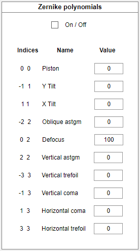
Each polynomial is calculated on the unitary disk, where the shorter side of the set resolution is taken as the disk diameter. By default, the function is restricted to 3rd-order Zernike polynomials, however, more complex holograms can be easily achieved by the combination of those available. As the result, the set of polynomials will be combined into the final hologram and superposed with other BCAA functions, in the control panel.

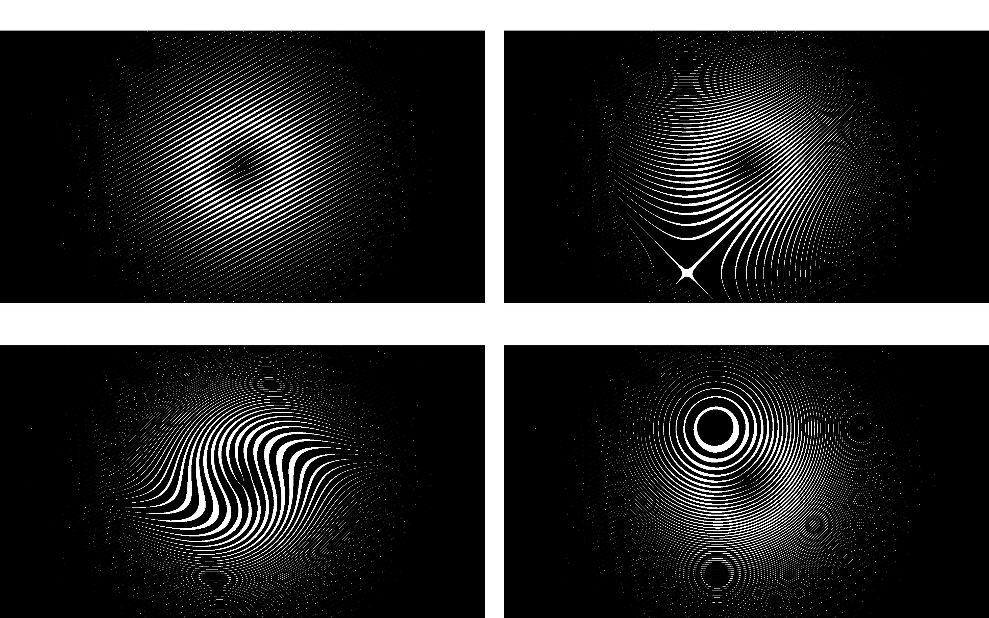
The examples of using Zernike polynomial are presented below: A) Laguerre-Gaussian beam p=0, l=1, beam waist=2; B) Laguerre-Gaussian beam p=0, l=1, beam waist=2 with Vertical astigmatism Value=100; C) Laguerre-Gaussian beam p=0, l=1, beam waist=2 with Vertical coma Value=100; D) Laguerre-Gaussian beam p=0, l=1, beam waist=2 with Defocuse Value=100. There is no necessary to use such a huge value, in real experimental setup affects of Zernike polynomials on real beam are noticeable for significantly smaller values (e.g. 1-10). But changes in amplitude hologramsthere are bearly seen, that’s why here values equal to 100 are implemented.