Laguerre-Cosinus & Laguerre-Sinus
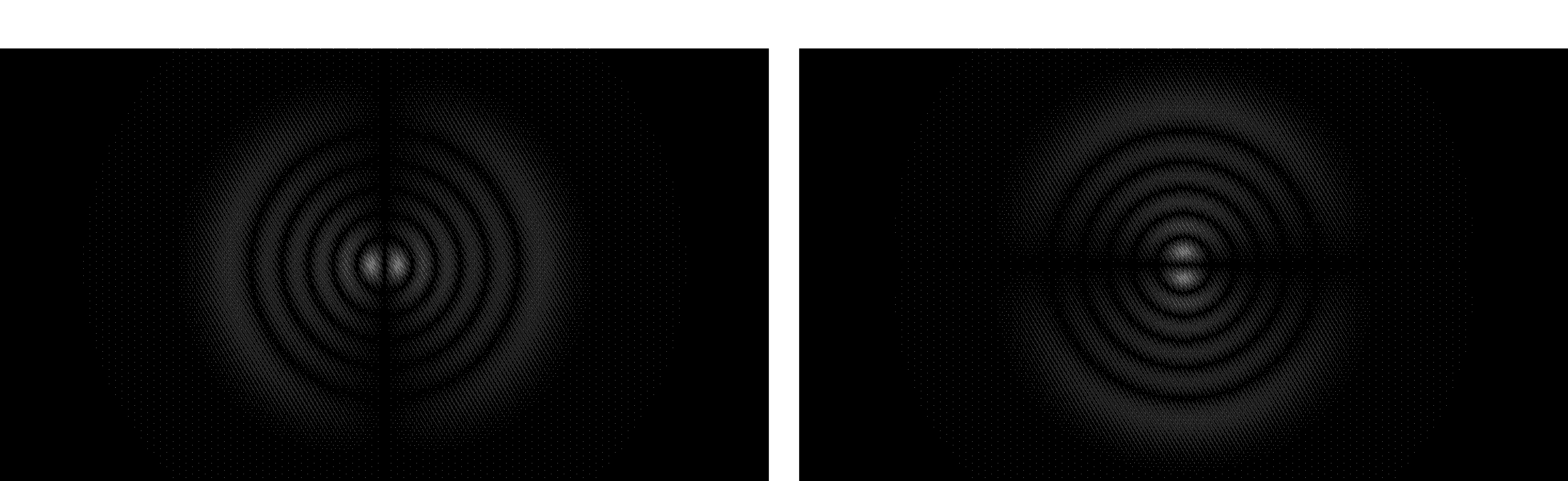
This functions are responsible for creating amplitude maps of Laguerre-Cosinus and Laguerre-Sinus beams [1].
\(LC^l_{p}=\frac{1}{\sqrt{2}}\left(\frac{\rho}{w_{0}}\right)^{|m|}\exp{\left[\frac{-\rho^2}{w_{0}^2}\right]}\mathbb{L}_{p}^l\exp{[jm\phi]}cos(l\phi),\)
\(LS^l_{p}=\frac{1}{\sqrt{2}}\left(\frac{\rho}{w_{0}}\right)^{|m|}\exp{\left[\frac{-\rho^2}{w_{0}^2}\right]}\mathbb{L}_{p}^l\exp{[jm\phi]}sin(l\phi),\)
where \(m\) is a topological charge, \(\mathbb{L}_{p}^l\) is Laguerre polynomial. The superposition of these two beams creates a Laguerre-Gaussian beam. Users can specify the azimuthal and radial indexes \(l,p\) in both cases. The presented examples shows the Laguerre-Cosinus (A) and Laguerre-Sinus (B) amplitude maps, both for the azimuthal index \(l = 1\) and radial index \(p = 5\).